Do you remember those picture puzzles “find X number of differences!”? Look at those pictures above but this time, without trying to find the differences. You probably didn’t realize all of the 7 differences in the first glance, right? So, if we don’t realize the differences at first glance, are they really important then? Is their difference “significant”?
This is where our journey begins.
Claiming The Difference!
During my industrial career, I’ve seen many people claiming that “our sales are now better than last year by xx percentage”, “this new design is giving better results”, “this supplier works better than the other supplier” etc. Yet, behind only very few of these sentences, I saw a solid “statistical” basis.
Let’s say, somebody said “our sales are better than last year by %5 after the launch of our new process”. What if it’s the same amount of sales with the sales of 2 years before without that process? Maybe there is already a “random” fluctuation which comes from many external effects like the economical situation in the country, fluctuation on the sales of rivals etc. But if the same person would say “Our sales are better by %70”, then we probably wouldn’t question those external factors that much in detail. Because the difference is simply “too large”.
A more specific example: You developed 2 versions of a drug let’s say Alpha and Beta. Alpha cured %31 of the test group, Beta cured %33. What if the people in Alpha test have some rare allergies which caused drug not to work properly and what if some portion of Beta tested people are cured just because of the placebo effect, not the Beta drug? Maybe in the perfect testing conditions, Alpha would have %35 curing rate and Beta would have %28. Yet, there is no such thing as perfect conditions! There is always some interference, some noise adding a “randomness” to our data.
Yet, if the difference would be %20 between those drugs, we wouldn’t question the effectiveness that much, right?
Big differences in numbers increases the trust or confidence!
Then, what is the threshold? Where do we start saying the difference is not coming from “the randomness” , it’s just simply a “significant difference”?
Testing the Difference (a.k.a Hypothesis Testing)
So, of course there is a way to say if your new data is really1 different or not. We can compare their averages by Student’s T-Test2 (a.k.a. just the T-Test) and we can statistically prove that these samples are different with a level of confidence.
So, if we are doing some test, there should be a kind of expectation from our test right? If you are performing a T-test, here below our competing hypothesis:
Default Expectation (a.k.a.\(H_0\)or Null Hypothesis) : The things you compare are NOT really different. They just seem different!
Opposite Expectation (a.k.a\(H_a\)or alternative Hypothesis) : There is a statistically significant difference between the compared things!
According to results of T-test, we can understand if our samples are significantly different or not.
Ingredients
To perform the T-test, we need:
Data or observations to compare.
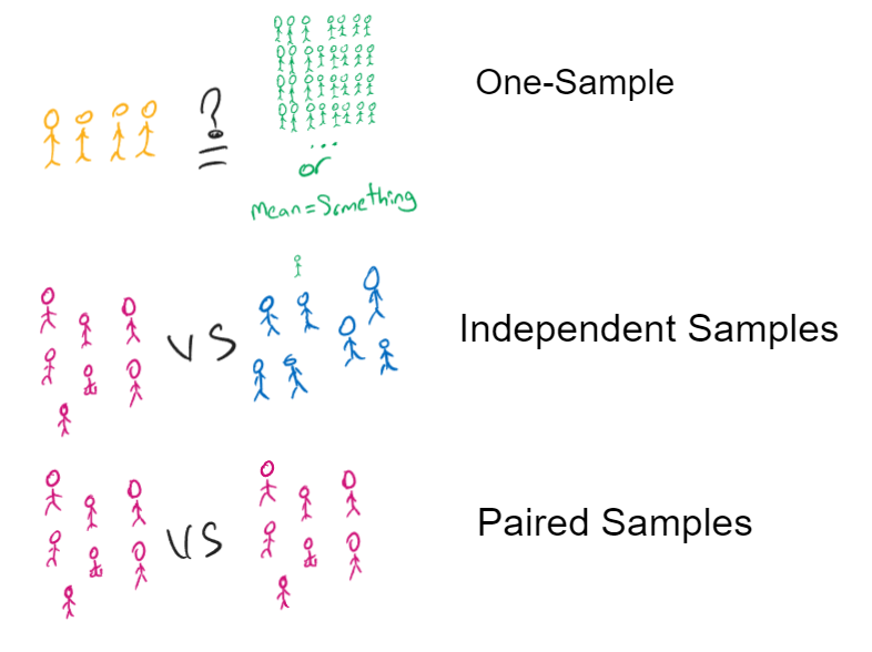
It can be one sample and we can compare it with a target value
It can be 2 samples which are totally independent from each other
It can be 2 samples which comes from related groups (can be same group, item or being subjected to same conditions)
As an output of the method’s calculation, a test statistic
A significance level
Degrees of freedom (\(df\))
Test statistic: A measure of how far the sample data deviates from the null hypothesis. (For T-test, it’s called T-Value)
Significance level: A threshold for determining whether the difference is statistically significant or just due to chance. It’s basically, the measure of “how confident we are” when we say it’s different or not.
Degrees of freedom : The number of independent pieces of information available after estimating one or more parameters from a sample of data. If you have 30 observations in your sample data, if you take any of the observations, there will be 29 other observations which carries independent information. In short, if your sample size is \(n\) , your \(df=n-1\).
Some Boring Terminology
Yeah, sorry. 😐 But at least, I will not go into mathematical details of the T-test because you will probably never need them. However, understanding the terms below is really important.
T-Value
When we run the T-test, we get a T-value. (suprise! 😝) This value is a measure of how different our average is from our target average or second sample. Then according to our significance level (let’s say 0.05 or %95) we will understand if we have a significant difference or not.
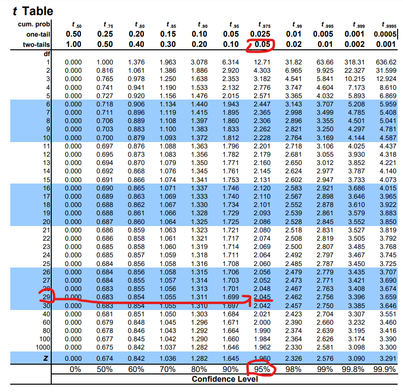
There is a table called T-Table and in this table, for some generally used confidence levels, threshold values of t-values are available. You can find your critical t-value in this table. If your t-value is beyond the critical t-value, then there is significant difference. If not, there is not!
Example: You have 30 samples, you need %95 confidence level (in other words, 0.05 significance level). So, your degrees of freedom is 29 and the critical t-value is 2.045.🚀
One-Tail / Two-Tails Thing
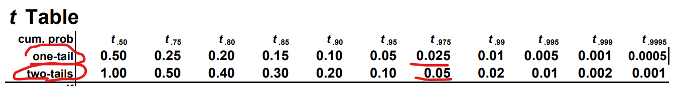
In the t-table, you may notice there are 2 different values and if the significance level 0.05 for two tails, it’s 0.025.
Why we need this? Because probability is changing depending of the question we ask.
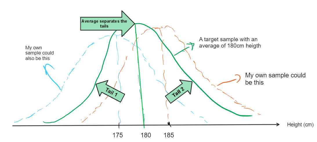
For example, we measure some men’s height and we want to understand if their average height is greater than 180cm or not. Let’s say, we found the probability of being greater than 180 as x. If we would ask the question like is it less than 180 or not, wouldn’t it be the same probability, which is x? If we say not greater, or not less, but just simply “if it’s different than 180 or not?”, then the probability of being different would be 2 times more.
In other words, if we ask the question as “is it greater” or “is it less” , we care the difference in only one-direction which means, we care only “one-tail” of a distribution. If we ask the question as “is it just different”, than we ask for “two-tails”.
P-Value
T-tests also generate another valuable information called p-value.
When we assume that there is no difference between our samples, the p-value tells us the probability of observing a t-value as extreme or more extreme than the t-value we calculated in our test.
Basically, it gives how are the odds to get this result. If the p-value is smaller than your significance level (usually 0.05 or %95 confidence level), it means that the difference between the compared averages cannot be explained by chance alone, in other words, the difference is statistically significant. On the opposite, if the p-value is larger than the significance level we chose, it means that there is a slight difference which could have come just by chance.
Steps
Longer way:
Run the test, get the T-value
Look to the t-table, find the critical t-value
Compare your t-value with the critical t-value. If your t-value is greater than the critical value, then there is a significant difference.
Shorter way:
Run the test, get the p-value.
Compare with your significance level and get your result. (i.e. If your confidence level is %95, your significance level is 1-0.95=0.05. So, if your p-value is greater than 0.05, there is no significant difference. If not, there is a significant difference.)
Running The Test
Running with R
If you use R, running the test is quite simple. You simply use the function called , wait for it, “t.test”! 😀
Hide / show the code
# Using a height data from MASS package, get the heights of maleslibrary(MASS)mens_height=na.omit(subset(survey$Height,survey$Sex=="Male"))# Let's take a random 30 sample from heightsset.seed(42)h.sample =sample(mens_height,30)# Run the testt.test(h.sample, # sample datamu=180, # Average we want to test against or target valueconf.level =0.95) # Confidence level we want
    One Sample t-test

data:  h.sample
t = -0.47037, df = 29, p-value = 0.6416
alternative hypothesis: true mean is not equal to 180
95 percent confidence interval:
 176.2777 182.3303
sample estimates:
mean of x
  179.304
Our p-value is 0.64 which is higher than 0.05. So, there is no statistically difference between our men heights and a sample which has an average value of 180cm height.
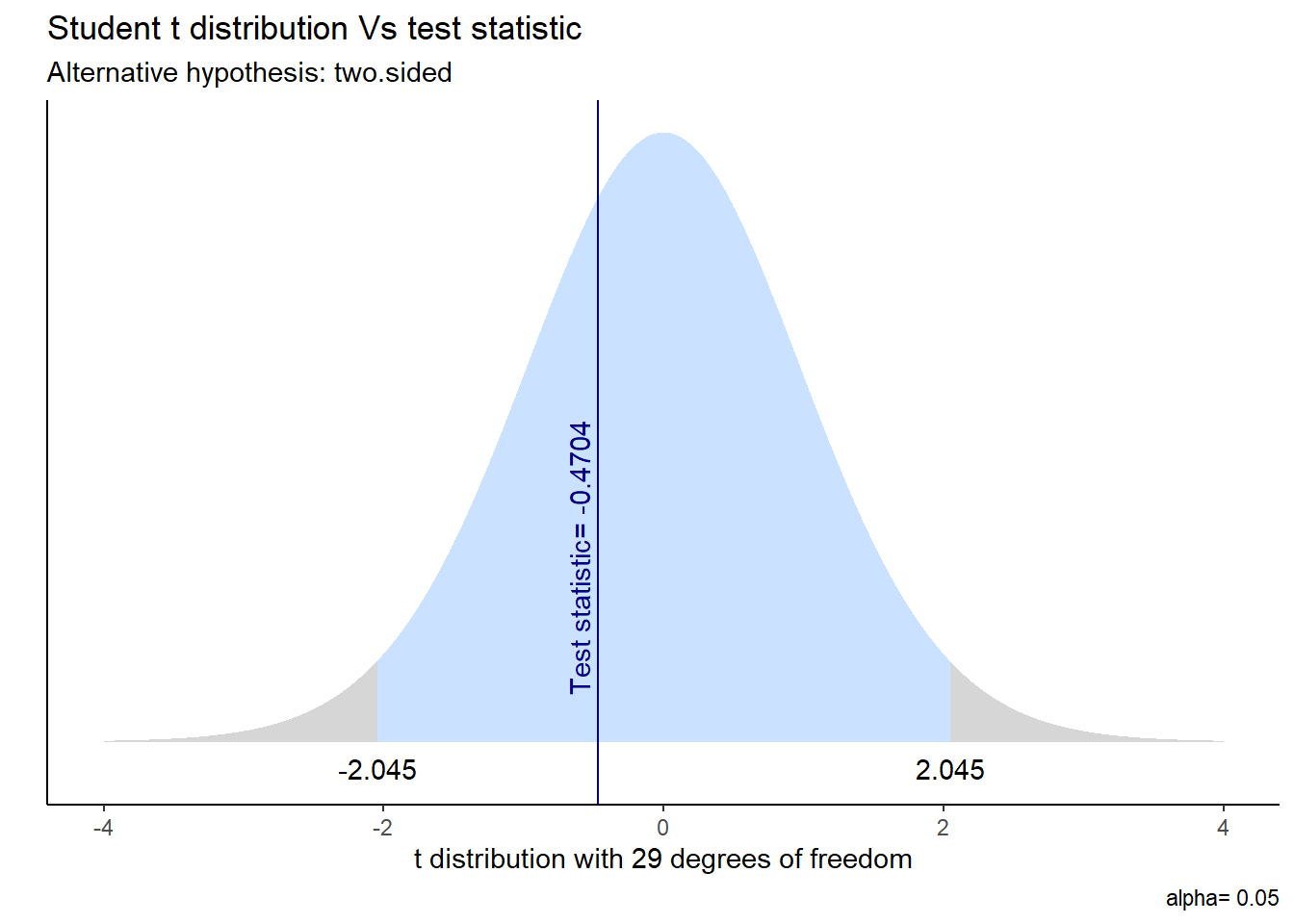
If you want to visualize it:
Did you recognize the “2.045” in this graph? No? C’mon, it was what we found in the t-table before! ⬆️ In other words, it was the critical t-value for two-tails %95 confidence level.
Since our t-value calculated as -0.4704, we can say the same: our data is not statistically significantly different than some population wihch has 180cm average height.
Running with Excel
There are 2 ways to get the same statistics in Excel:
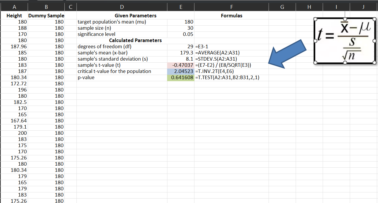
1- Excel formulas
You can use the t-value mathematical formula and the formulas given below, you will get the same results.
By using Analysis Toolpak3, you can get the same statistics as shown below:
Wrap-up and Notes
T-test is one of the hypothesis tests but not the only one.
T-test can compare the averages of 2 samples or 1 sample against a target value and give you if the difference is statistically significant or not.
T-test also have some assumptions before you perform it:
The data in each group should be approximately normally distributed.
The samples you compare are continuous data. (Not something like Fail/pass or proportional data)
Since it’s a simple mathematical formula, you can run it even your old school calculator. But inside the tools like Excel or R, there are already embedded functions for this.
Going Further
Now that you understand the basics of hypothesis testing and even already seen one example of it.
But what if your data is not normally distributed? How will you even know if it’s normally distributed or not?What if your data is not continuous like height but you want to compare a proportion instead?
Here are some common hypothesis tests and brief explanations of them (we only talked about first 3 in this article:
One-sample t-test: used to test whether a population mean is equal to a specified value.
Two-sample t-test: used to test whether the means of two independent samples are significantly different.
Paired t-test: used to test whether the means of two related samples are significantly different.
One-way ANOVA: used to test whether the means of three or more independent groups are significantly different.
Kruskal-Wallis test: a non-parametric alternative to one-way ANOVA for testing differences in medians among three or more independent groups.
Chi-square test of independence: used to test whether there is a significant association between two categorical variables.
Chi-square goodness of fit test: used to test whether the observed frequency distribution of a categorical variable differs from a hypothesized frequency distribution.
Binomial test: used to test whether the proportion of successes in a sample of binary data is significantly different from a hypothesized proportion.
Wilcoxon signed-rank test: a non-parametric alternative to paired t-test for testing whether the medians of two related samples are significantly different.
Mann-Whitney U test: a non-parametric alternative to two-sample t-test for testing whether the medians of two independent samples are significantly different.
As you see, there seem to be lots of different tests but the logic is always similar.
We can talk more on these if someone put’s a comment below to talk about them. Otherwise, maybe it’s the best to stop at here. 🤭
See ya folks! 🤠
Footnotes
In statistical jargon: statistically significant↩︎
In 1908 William Sealy Gosset, an Englishman publishing under the pseudonym Student, developed the t-test and t distribution. For more: https://www.britannica.com/science/Students-t-test↩︎