Hide / show the code
# R way of loading the library
library(tidyverse)
I’m posting this because I would like to sincerely help the others who are struglling to switch to Python after learning R. (Because if you started with R, you will probably learn Python at some point, believe me. 😁)
Also, this will be a loooong post but I don’t expect you to read line by line. My intention is to turn this document as a head start document which you can come back and check what was the basic equivalents of these functions.
Shall we begin?⛷️
First of all I’m not gonna talk about why I had to learn Python as well as a R Programmer. You can find tons of videos about that online. Yet, I think it’s worth to discuss the ‘bridge’ points to make it easier for the people who are on the similar path.
By the way, I will be running everything in this post directly inside R-Studio and Quarto thanks to great library called reticulate made by Posit developers.
Choosing the IDE is one of the most important starting steps I believe. Because no matter how good you are in a particular language, learning an IDE takes time, really. So, if you do it wrong in the beginning, you may end up learning another one from the beginning.
For R, the choices are not that much already! R-Studio is far most the best for R.
However, when it comes to python, some will say go with Anacondaand Spyder, some will say use PyCharm… Most of the tutorials are on Jupyter notebooks… Some will also say go for google colab… I’m not even talking about the other platforms like Atom.
There could be tons of resources and maybe much better ones but, as a R programmer, I highly recommend for you to use VS Code! Simply because:
But really, I wanna talk more about some point: Wanna go with jupyter notebook? It runs it… Standard python files? Easy! Wanna write some R code on the side, even with Quarto or Rmarkdown? Nooo big deal. It just supports everything you can imagine and this flexibility is just great!
It’s a little bit different than other IDE’s I’ve used and sometime taking time to find out where are the things but after you get used to it, it’s one of the best choices out there.
Wanna start with VS Code? A nice place to start is the video down below:
Before going further, I would like to give a simple trick for the people who knows and uses %>% in R. If you don’t know that symbol, you can just skip this part.
%>% operator, a.k.a. pipe, does a very simple, yet powerful job in R which links the outputs of separate functions to each other. It’s creating an information flow or a chain and each output is passed to the next function to let us work with it. This is great, because it’s saving us creating a lot of unnecessary and temporary variables one by one for each function.
Good news is, this is actually how python works, too, even without any additional library!
So, if you know how to use %>% , then you are already done understanding how python method approach is working!
Look at this example of getting standard deviation in both languages:
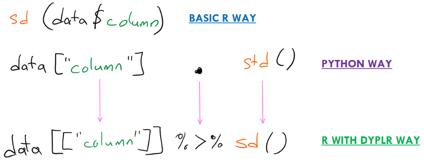
If you go with standard R way, it can be complicated to make the link but if I switch to dyplr and change my way of adressing the columns, it’s the same approach!
In R, we usually don’t use :: sign while our coding but we know it’s there, just taking care by R after we load the library. But, it’s not the case in python. You need to use
# R way of loading the library
library(tidyverse)# Python way of loading the library
import pandas as pdAs you can see, even if it’s not easy as R, Python has a way of at least making easier to code with libraries by using ALIAS. as pd part is defining that. We will save some typing by writing pd instead of pandas at least. 😝
This part is similar. But unlike R, there is a native support of Python to read xls or csv.
# R way
library(readr)
mydata <- read_csv("CardioGoodFitness.csv")# Python way
mydata = pd.read_csv('CardioGoodFitness.csv')This is one of the good parts which I see not much difference but let’s look to the head - tail first:
head(mydata,3)# A tibble: 3 × 9
Product Age Gender Education MaritalStatus Usage Fitness Income Miles
<chr> <dbl> <chr> <dbl> <chr> <dbl> <dbl> <dbl> <dbl>
1 TM195 18 Male 14 Single 3 4 29562 112
2 TM195 19 Male 15 Single 2 3 31836 75
3 TM195 19 Female 14 Partnered 4 3 30699 66tail(mydata,3)# A tibble: 3 × 9
Product Age Gender Education MaritalStatus Usage Fitness Income Miles
<chr> <dbl> <chr> <dbl> <chr> <dbl> <dbl> <dbl> <dbl>
1 TM798 45 Male 16 Single 5 5 90886 160
2 TM798 47 Male 18 Partnered 4 5 104581 120
3 TM798 48 Male 18 Partnered 4 5 95508 180mydata.head(3) Product Age Gender Education MaritalStatus Usage Fitness Income Miles
0 TM195 18 Male 14 Single 3 4 29562 112
1 TM195 19 Male 15 Single 2 3 31836 75
2 TM195 19 Female 14 Partnered 4 3 30699 66mydata.tail(3) Product Age Gender Education MaritalStatus Usage Fitness Income
177 TM798 45 Male 16 Single 5 5 90886 \
178 TM798 47 Male 18 Partnered 4 5 104581
179 TM798 48 Male 18 Partnered 4 5 95508
Miles
177 160
178 120
179 180 The biggest difference comes with the . notation in Python. Because in R, we are so used to use () with functions. But this it both good and bad actuallly.
function. (In python, after the . , you can also call the variable name for instance)%>% with dplyr library.In R, we can get 5 Points summary using summary function:
# Summary on R
summary(mydata)
Product Age Gender Education
Length:180 Min. :18.00 Length:180 Min. :12.00
Class :character 1st Qu.:24.00 Class :character 1st Qu.:14.00
Mode :character Median :26.00 Mode :character Median :16.00
Mean :28.79 Mean :15.57
3rd Qu.:33.00 3rd Qu.:16.00
Max. :50.00 Max. :21.00
MaritalStatus Usage Fitness Income
Length:180 Min. :2.000 Min. :1.000 Min. : 29562
Class :character 1st Qu.:3.000 1st Qu.:3.000 1st Qu.: 44059
Mode :character Median :3.000 Median :3.000 Median : 50597
Mean :3.456 Mean :3.311 Mean : 53720
3rd Qu.:4.000 3rd Qu.:4.000 3rd Qu.: 58668
Max. :7.000 Max. :5.000 Max. :104581
Miles
Min. : 21.0
1st Qu.: 66.0
Median : 94.0
Mean :103.2
3rd Qu.:114.8
Max. :360.0 For the same, there is a built-in method called describe in Python.
# Summary on Python
mydata.describe(include="all")
Product Age Gender Education MaritalStatus Usage
count 180 180.000000 180 180.000000 180 180.000000 \
unique 3 NaN 2 NaN 2 NaN
top TM195 NaN Male NaN Partnered NaN
freq 80 NaN 104 NaN 107 NaN
mean NaN 28.788889 NaN 15.572222 NaN 3.455556
std NaN 6.943498 NaN 1.617055 NaN 1.084797
min NaN 18.000000 NaN 12.000000 NaN 2.000000
25% NaN 24.000000 NaN 14.000000 NaN 3.000000
50% NaN 26.000000 NaN 16.000000 NaN 3.000000
75% NaN 33.000000 NaN 16.000000 NaN 4.000000
max NaN 50.000000 NaN 21.000000 NaN 7.000000
Fitness Income Miles
count 180.000000 180.000000 180.000000
unique NaN NaN NaN
top NaN NaN NaN
freq NaN NaN NaN
mean 3.311111 53719.577778 103.194444
std 0.958869 16506.684226 51.863605
min 1.000000 29562.000000 21.000000
25% 3.000000 44058.750000 66.000000
50% 3.000000 50596.500000 94.000000
75% 4.000000 58668.000000 114.750000
max 5.000000 104581.000000 360.000000 Also table function to get a contingency table easily:
# Contingency Table on R
table(mydata$Gender, mydata$Product)
         TM195 TM498 TM798
  Female    40    29     7
  Male      40    31    33
The same is possible with describe and crosstab functions in pandas in Python.
# Contingency Table on Python
pd.crosstab(mydata['Gender'],mydata['Product'])
Product TM195 TM498 TM798
Gender
Female 40 29 7
Male 40 31 33We can have a glimpse in R on data as below:
# Glimpse with R
glimpse(mydata)
Rows: 180
Columns: 9
$ Product <chr> "TM195", "TM195", "TM195", "TM195", "TM195", "TM195", "T…
$ Age <dbl> 18, 19, 19, 19, 20, 20, 21, 21, 21, 21, 22, 22, 22, 22, …
$ Gender <chr> "Male", "Male", "Female", "Male", "Male", "Female", "Fem…
$ Education <dbl> 14, 15, 14, 12, 13, 14, 14, 13, 15, 15, 14, 14, 16, 14, …
$ MaritalStatus <chr> "Single", "Single", "Partnered", "Single", "Partnered", …
$ Usage <dbl> 3, 2, 4, 3, 4, 3, 3, 3, 5, 2, 3, 3, 4, 3, 3, 3, 2, 4, 4,…
$ Fitness <dbl> 4, 3, 3, 3, 2, 3, 3, 3, 4, 3, 3, 2, 3, 3, 1, 3, 3, 3, 3,…
$ Income <dbl> 29562, 31836, 30699, 32973, 35247, 32973, 35247, 32973, …
$ Miles <dbl> 112, 75, 66, 85, 47, 66, 75, 85, 141, 85, 85, 66, 75, 75…While the similar approach is possible with the Python built-in method info() :
# Glimpse with Python
mydata.info()
<class 'pandas.core.frame.DataFrame'>
RangeIndex: 180 entries, 0 to 179
Data columns (total 9 columns):
# Column Non-Null Count Dtype
--- ------ -------------- -----
0 Product 180 non-null object
1 Age 180 non-null int64
2 Gender 180 non-null object
3 Education 180 non-null int64
4 MaritalStatus 180 non-null object
5 Usage 180 non-null int64
6 Fitness 180 non-null int64
7 Income 180 non-null int64
8 Miles 180 non-null int64
dtypes: int64(6), object(3)
memory usage: 12.8+ KBWe see also memory usage with info which can be handy for large datasets.
# Get the memory usage of the data frame
object.size(mydata)
21096 bytesBy the way, for same dataset, while Python uses 12.8KB roughly, R uses around 20KB. This difference could be coming from the power of pandas. Yet, it’s an interesting fact which can give some hints what’s gonna be on the performance comparison between Python and R especially for large datasets.
Of course one of the must have summaries is grouped aggregations or pivot tables.
In R, one of the most common ways to create a pivot table is to simply do it by dyplr. Yet, I can say, it’s not a great way, though.
# Pivot table in R
mydata %>%
  group_by(Product, Gender, MaritalStatus) %>%
  summarize(count = n()) %>%
  spread(MaritalStatus, count)
`summarise()` has grouped output by 'Product', 'Gender'. You can override using
the `.groups` argument.# A tibble: 6 × 4
# Groups: Product, Gender [6]
Product Gender Partnered Single
<chr> <chr> <int> <int>
1 TM195 Female 27 13
2 TM195 Male 21 19
3 TM498 Female 15 14
4 TM498 Male 21 10
5 TM798 Female 4 3
6 TM798 Male 19 14Pandas provides a simpler way on Python side. The way of creating it is quite similar how we do it in Excel.
pd.pivot_table(mydata, index=['Product', 'Gender'],
                       columns=[ 'MaritalStatus'], aggfunc=len)
Age Education Fitness Income
MaritalStatus Partnered Single Partnered Single Partnered Single Partnered
Product Gender
TM195 Female 27 13 27 13 27 13 27 \
Male 21 19 21 19 21 19 21
TM498 Female 15 14 15 14 15 14 15
Male 21 10 21 10 21 10 21
TM798 Female 4 3 4 3 4 3 4
Male 19 14 19 14 19 14 19
Miles Usage
MaritalStatus Single Partnered Single Partnered Single
Product Gender
TM195 Female 13 27 13 27 13
Male 19 21 19 21 19
TM498 Female 14 15 14 15 14
Male 10 21 10 21 10
TM798 Female 3 4 3 4 3
Male 14 19 14 19 14 I think Python way is much more intuitive than R. Especially group_by() %>% summarize() combination could be pretty confusing for beginners. Because, if you don’t add summarize() , group_by is doing the grouping in the back, you even don’t realize it’s gonna stay grouped that way. You need yo ungroup after to avoid problems later. (If anyone knows a specific library for pivot table, please feel free to share and I will update here. 😉)
mydata[["Age"]] %>% sd()[1] 6.943498When it comes to graphs, we have our basic plot , hist or boxplot kind of basic visualizations in R which I find usually very ugly! 😝 Yet, we have also our beautiful ggplot and plotly, yay!
In python, for me, basics go with the matplotlib which is actually derived from my old pal MATLAB and for fancier graphs, there is seaborn library. Yet, one the the greatest news on this, both Python and R supports plotly! 👍😍
Sooo, let’s dive-in!
to be continued….