Let’s think that you are making sampling from Boston Housing dataset and you are separating your dataset into 2 sets as training and test sets.
Ideally, you need to pick the variables “randomly” to have a healthy training and test sets. So, in terms of Boston Housing set, let’s say, you randomly picked up 150 observations for your test set and 356 observations for your training set. (There are 506 obs. in total) What if you partition the data like most of the cheap and moderate houses are in training and most of the expensive ones are in the test set? Another example: let’s say you have a biological data which also contains gender in one column. What if your training set would be mostly male observations and test set mostly based on females?
That’s why, it’s very important to ensure that the model is trained and tested on a “representative sample” of the population. This will help to reduce bias in our models. Otherwise, it would be like you are making a survey on voting then you are making a prediction algorithm mostly based on A party followers but testing it on mostly B party follower responses.
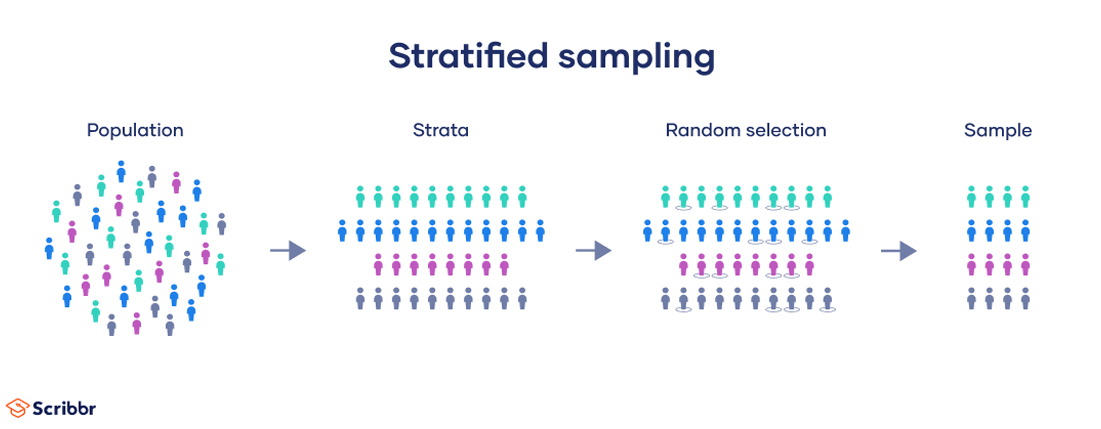
The process of enrusing that our samples of both training and test sets are “representative samples” is called “Stratified Sampling”.
Simply you are grouping your data in the groups which called “strata”. Then you are doing your random selections from each group as proportionally equal as possible.
3 How to do In R?
3.1 1- Creating the “Strata”s
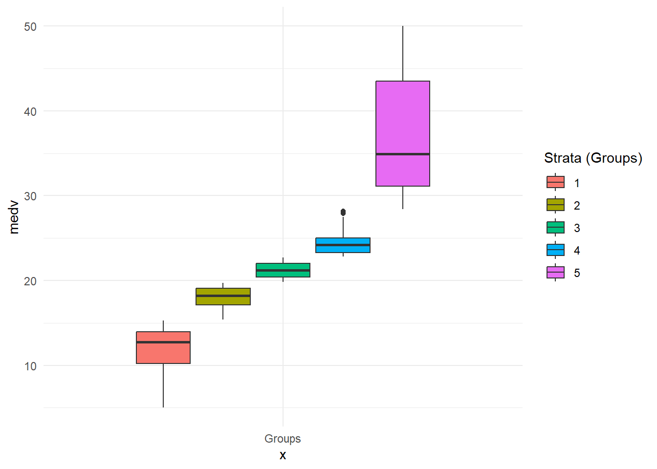
Let’s say you are working on Boston Housing. In this dataset, main variable is median value of houses which is called “medv”. Since it’s price, which is a continuous number, how we can group it? We can simply think it as “distribution” and we can divide it into 5 slices as the data quantiles and we can be sure that when R is taking the samples, it can pick 1 from each group instead of blindly randomizing. Therefore, we can start by using cut function and dividing the data with this quartiles. Just for practice purpose, I’m also going to plot it.
Hide / show the code
# Loading the libraries-----------------------------------------------------if (!require("pacman")) install.packages("pacman")
Loading required package: pacman
Hide / show the code
p_load(pacman, MASS, rsample, tidyverse)# --------------------------------------------------------------------------# Take boston dataset to a dataset tabledataset.df <- Boston# Fix the random numbers by setting the seed set.seed(42)# Create a strata or grouping column based on distribution quantilesstrata <-cut(dataset.df$medv,breaks =quantile(dataset.df$medv, # putting the response variable# creating probability slices like 0-%20,%20-40...probs =seq(0, 1, 0.2)), # Should it include the values on breaks like the one in %20? YES!include.lowest =TRUE,# Do I need labels like "0-15.1, 15.1- 30.2" or integer as "1,2,3"?# FALSE means: Go with the integer! :) labels =FALSE)# Let's add these groups to our main data and check temp1 <-cbind(dataset.df, strata)# Plottt!ggplot(temp1) +aes(x ="Groups", y = medv, fill =as.factor(strata), group = strata) +geom_boxplot() +theme_minimal() +labs(fill="Strata (Groups)")
So, as we see, each strata or group starts after the point the next one begins. If we would randomly pick the values from each colored areas equally, we would expect naturally that test and training set distributions will be very close to each other.
3.2 2- Using Stratas in the Sampling
We can use initial_split in rsample library.
Hide / show the code
data_split <-initial_split( temp1, # the temporary datset we created - it has the "strata" prop =0.70, # I schoe %70 / %30 ratio# We are choosing our new column "strata" for groupingstrata="strata") # Create data frames for the two sets# (excluding the strata variable with "[,-ncol(temp1)]", we don't need it anymore)train.df <-training(data_split)[,-ncol(temp1)] test.df <-testing(data_split)[,-ncol(temp1)]
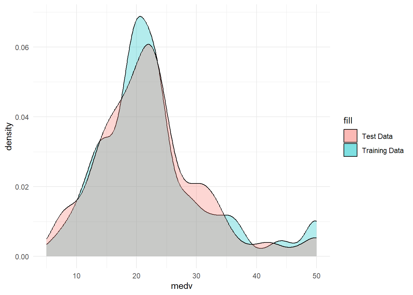
initial_split is taking a randomized sample but it also used in its process the groups we created. Now, we can check if it worked or not:
ggplot() +geom_density(data=train.df, adjust = 1L, alpha=0.3,aes(x= medv, fill ="Training Data")) +geom_density(data=test.df, adjust = 1L, alpha=0.3,aes(x= medv, fill ="Test Data")) +theme_minimal()
Yes! Our test and training set distributions are pretty close to each other!
3.3 Conclusion
Just to simplyfy it, I’m merging all the code as below. But you need to remember that, sometimes you could be in need of more than 1 strata. So, you need to create your sub groups accordingly and use in the function with the “c(var1,var2…)” type of syntax.
Here is the code and see you on the next study! 😇
Hide / show the code
# Loading the libraries-----------------------------------------------------if (!require("pacman")) install.packages("pacman")p_load(pacman, MASS, rsample, tidyverse)# --------------------------------------------------------------------------# Take boston dataset to a dataset tabledataset.df <- Boston# Fix the random numbers by setting the seed set.seed(42)# Create a strata or grouping column based on distribution quantilesstrata <-cut(dataset.df$medv, breaks =quantile(dataset.df$medv, probs =seq(0, 1, 0.2)), include.lowest =TRUE, labels =FALSE)# Add these groups to our main data and check temp1 <-cbind(dataset.df, strata)# Creating the splitdata_split <-initial_split( temp1,prop =0.70,strata="strata") # Create data frames for the two setstrain.df <-training(data_split)[,-ncol(temp1)] test.df <-testing(data_split)[,-ncol(temp1)]